Explaining the Now-cast, redux.

This post is for those true data geeks who want the real nitty-gritty of how I am trying to reduce the lag on San Francisco’s case numbers from 10 days to 3 days. If you are interested in this or have questions please don’t hesitate to reach out to me. Please if you see ways of improving the projections I’m making feel free to suggest them.
This is my second attempt at “forecasting” (maybe we call it after-casting) what results from 3 days ago will look like 4 days from now. In this go round I tried to add an estimation of error to give us all a sense of the range in which the now-cast should be accurate.
First the problems
Built in 3 day lag- San Francisco’s new case data always lags by 3 days. The most recent new case specimen collection dates entered for San Francisco are at least three days old. Unless San Francisco starts updating their database more quickly I can’t get past this barrier.
Another 3 days for cases to build up- Only a small fraction of cases are reported with only 3 days delay. Many more positive tests arrive on day 4 and day 5. By day 6 almost all the cases for a particular specimen collection date have been logged.
Another 4 days for weekly averaging- The daily case numbers are too noisy to spot trends. The weekend weekday disparity I’ve discussed previously contributes mightily to this problem. To overcome this I use a weekly average. (ie to calculate the case rate for a particular day on my curves I average that day with the 3 days before and after this day.) This introduces another 3 days of lag into the case rate.
This is a total of ten days which I wanted to bring down as far as I could, ideally three days.
Projecting the build up of cases.
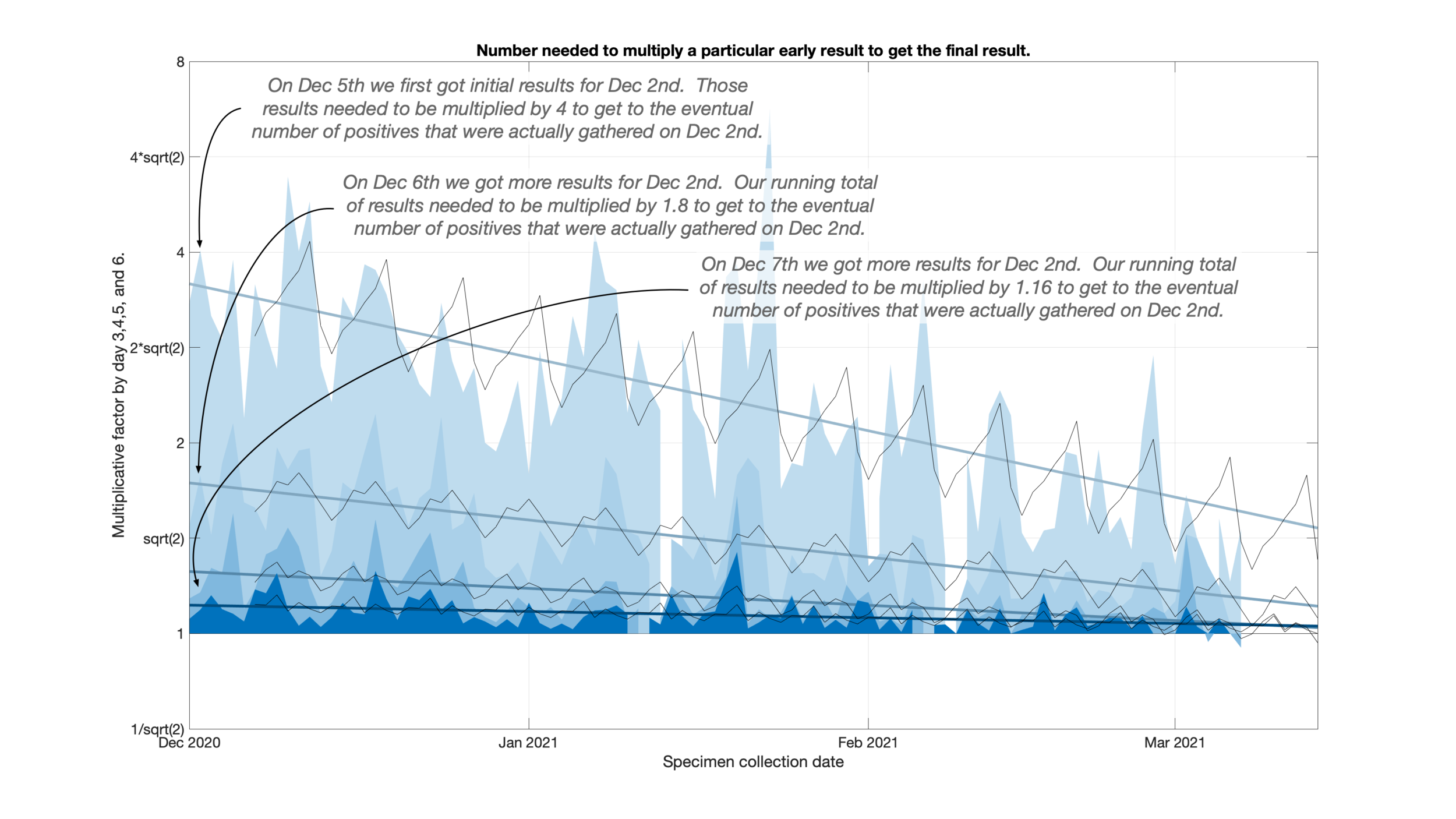
Looking back at the failure of my previous prediction I noticed that the testing delays were consistently dropping. This meant that results would show up earlier than they used to but my previous algorithm would think that more results were still yet to arrive. I was over estimating where the eventual positive count would end up.
I fit a line to a set of factors to take improvements in testing delays into account. As a side benefit you can really see how testing delays have fallen over the past couple of months.
Because test sites seem to have weekly testing schedules, I also allowed for a variation by day of the week to appear on top of this trend line.
Well into the weeds here- The number being fit is the number that a particular very recent day needs to be multiplied by to get to the eventual total many days later. Ie how close is the most recent result to the total.
Even more into the weeds- I actually fit the log base 2 of the multiplicative factor so that a multiplication by 2 and a multiplication by 1/2 would “average” to 1.
Weekly average adjustments. Done as an example.
I average over the course of a week to smooth out the variation in the amount of testing on the various days of the week.
For the recent days I do not have a week’s worth of data to average over. I take a subset of the data and compare it to the same subset in the previous week.
For example I downloaded the SF dataset on March 14th. The most recent day of COVID-19 data is March 11th. From the section above I’ve estimated that the number of positives on March 11th need to be multiplied by 2 to get close close to their eventual total. In a similar fashion I multiply the positives given for March 10th, 9th, and 8th by a decreasing series of numbers bigger than 1. I now have an estimate for what these numbers will eventually be.
To get the weekly average for March 14th I look at how much this total has dropped or increased from the March 7th value a week earlier. I then multiply the weekly average for March 7th by this rise or fall to get my estimate for the weekly average.
To get the weekly average for March 13th I average March 12th, 13th, and 14th together and compare to March 5th, 6th, and 7th from the week before. I then multiply the weekly average of March 6th by this factor to get the new value for March 13th.
My code
Instead of trying to write more I’ll just put up my Matlab code and allow people to examine it.
% The first part of this script loads my old data from a matlab file and
% then loads any new data from recent days.
load core_reporting_data
covid_tx = sortrows( covid_tx, {'SpecimenCollectionDate'});
% Sanity check ***
% We expect that reports from older than 10 days prior to the previous
% reporting date wouldn't have changed much. Let's check to see if that's the
% case
previous_date = max( covid_tx.reporting_date);
stable_date = previous_date - 10;
stable_totals_l = (covid_tx.SpecimenCollectionDate <= stable_date);
last_report_l = (covid_tx.reporting_date == previous_date);
% Get the newest data which I keep in the source_data folder
new_covid_tx = add_to_tx_reporting_evolution( previous_date, '../source_data');
new_covid_tx = sortrows( new_covid_tx, {'SpecimenCollectionDate'});
new_totals_l = (new_covid_tx.SpecimenCollectionDate <= stable_date);
most_recent_l = (new_covid_tx.reporting_date == max( new_covid_tx.reporting_date));
if ~all( covid_tx.SpecimenCollectionDate( stable_totals_l & last_report_l) == new_covid_tx.SpecimenCollectionDate( new_totals_l & most_recent_l))
fprintf('Date mismatch\n')
keyboard
end
changed_idxs = find(covid_tx.totals( stable_totals_l & last_report_l) ~= new_covid_tx.totals( new_totals_l & most_recent_l));
if ~isempty( changed_idxs)
specimen_dates = covid_tx.SpecimenCollectionDate( stable_totals_l & last_report_l);
old_totals = covid_tx.totals( stable_totals_l & last_report_l);
new_totals = new_covid_tx.totals( new_totals_l & most_recent_l);
for ith_change = 1:length( changed_idxs)
delta_change = new_totals( changed_idxs( ith_change)) - old_totals( changed_idxs( ith_change));
fprintf('%s new total %3d delta from old %3d\n', ...
specimen_dates( changed_idxs( ith_change)), new_totals( changed_idxs( ith_change)), delta_change);
end
end
% Tack on the newest data to the earlier data
covid_tx = [covid_tx; new_covid_tx];
covid_tx = sortrows( covid_tx, {'SpecimenCollectionDate'});
% The line below adds an additional column to the matlab table
% so I now for most days since last summer have all the numbers reported.
% As I write this on March 13th this table is currently 58462 rows with the
% following columns and an example couple of rows
% SpecimenCollectionDate Community FromContact Unknown totals interviewed reporting_date days_delay
% ______________________ _________ ___________ _______ ______ ___________ ______________ __________
%
% 2020/03/03 2 0 0 2 2 16-Jul-2020 135
% 2020/03/03 2 0 0 2 2 17-Jul-2020 136
% 2020/03/03 2 0 0 2 2 18-Jul-2020 137
covid_tx.days_delay = days( covid_tx.reporting_date - covid_tx.SpecimenCollectionDate);
early_data_l = covid_tx.days_delay <= 6;
early_data = covid_tx( early_data_l, {'SpecimenCollectionDate','totals','days_delay'});
early_data_unstack = unstack( early_data, 'totals', 'days_delay');
now_date = max( covid_tx.reporting_date);
now_l = covid_tx.reporting_date == now_date;
most_recent_data = covid_tx( now_l, {'SpecimenCollectionDate','totals'});
full_data = join( early_data_unstack, most_recent_data);
full_data = full_data( full_data.SpecimenCollectionDate >= datetime( 2020, 9, 6), :);
full_data = sortrows( full_data, 'SpecimenCollectionDate');
% At this point in the code full_data is a table 185 rows by the following
% 7 columns. Below is an example. The column x3 is the total count at 3
% days delay, x4 at 4 days delay ... and the totals column is the number
% eventually reached.
% SpecimenCollectionDate x2 x3 x4 x5 x6 totals
% ______________________ ___ ___ ___ ___ ___ ______
%
% 2020/09/06 NaN 12 24 24 26 25
% 2020/09/07 NaN 19 50 47 48 49
% 2020/09/08 NaN 33 62 63 66 68
% This is the amount we need to multiply the early result by to reach the
% eventual total. It is more stable to multiply by a factor than to
% divide.
mult_factor = repmat( full_data.totals, 1, 4) ./ table2array( full_data(:, {'x3','x4','x5','x6'}));
% I use the logarithm of the multiplicative factor so that 2 and 1/2
% average to 1.
mult_factor_log2 = log2( mult_factor);
% This is a sanity check figure for me to eyeball to make sure that my
% fitting factors are appropriate.
matlab_blue = [0 0.4470 0.7410];
dark_blue = [0 0.3 0.5];
matlab_red = [0.8500 0.3250 0.0980];
figure(2)
clf
start_of_fit = datetime( 2020, 12, 1);
since_dec_l = ( full_data.SpecimenCollectionDate >= start_of_fit);
very_recent_l = (full_data.SpecimenCollectionDate >= (max( covid_tx.reporting_date) -7));
for column_of_interest = 1:4
nan_l = isnan( mult_factor_log2( :, column_of_interest));
fx3 = fit( days( full_data.SpecimenCollectionDate( since_dec_l & ~very_recent_l & ~nan_l) - start_of_fit), ...
mult_factor_log2(since_dec_l & ~very_recent_l & ~nan_l,column_of_interest), 'poly1');
ah = area( full_data.SpecimenCollectionDate(1:end-3), mult_factor_log2(1:end-3,column_of_interest));
ah.FaceColor = (matlab_blue + (4-column_of_interest)*[1 1 1])/(5-column_of_interest);
ah.EdgeAlpha = 0;
days_elapsed = days(datetime('today') - start_of_fit);
hold on
plot( [start_of_fit datetime('today')], fx3.p1 * [0 days_elapsed] + fx3.p2, ...
'-', 'LineWidth', 3, 'Color', (dark_blue + (4-column_of_interest)*[1 1 1]/2)/(3-column_of_interest/2))
end
%area( repmat( full_data.SpecimenCollectionDate(1:end-3), 1, 4), mult_factor(1:end-3,:))
grid on
xlim([start_of_fit datetime('today')])
xlabel('Specimen collection date')
ylabel('Multiplicative factor by day 3,4,5, and 6.')
set(gca,'FontSize',16)
% gather the numbers into weeks and average over the weeks.
% We need to be careful that if there's a day with a NaN that we throw out
% the value and properly average.
start_of_fit = datetime( 2020, 12, 1);
end_of_fit = (max( covid_tx.reporting_date) -7);
% We want to round down to get the number of days to fit into a fixed
% number of weeks
num_weeks_of_fit = floor( days( end_of_fit - start_of_fit) / 7);
excess_days = days( end_of_fit - start_of_fit) - (num_weeks_of_fit * 7);
start_of_fit = start_of_fit + excess_days +1;
weekly_fit_l = (full_data.SpecimenCollectionDate <= end_of_fit) & ...
(full_data.SpecimenCollectionDate >= start_of_fit);
% Average the days within the week taking care to average only 6 days if a
% day doesn't have data.
mult_factor_log2 = mult_factor_log2( weekly_fit_l, :);
mult_factor_log2 = reshape( mult_factor_log2, 7, num_weeks_of_fit, 4);
mult_factor_weekly_avg = mean( mult_factor_log2, 1, 'omitnan');
mult_factor_weekly_avg = reshape( mult_factor_weekly_avg, num_weeks_of_fit, 4);
% Now fit the weekly data
mult_factor_weekly_fit = NaN * ones( (num_weeks_of_fit+1)*7, 4);
for column_of_interest = 1:4
weekly_fit = fit( ((1:num_weeks_of_fit)'-1)*7, mult_factor_weekly_avg( :,column_of_interest), 'poly1');
mult_factor_weekly_fit( :, column_of_interest) = weekly_fit.p1 * ((1:((num_weeks_of_fit+1)*7))'-4) + weekly_fit.p2;
end
% Find daily difference between weekly fit
% This produces the daily variation on top of the weekly fit.
mult_factor_weekly_fit_trunc = reshape( mult_factor_weekly_fit((1:(num_weeks_of_fit*7)),:), 7, num_weeks_of_fit, 4);
mult_factor_delta = mean( mult_factor_log2 - mult_factor_weekly_fit_trunc, 2, 'omitnan');
mult_factor_delta = repmat( mult_factor_delta, 1, num_weeks_of_fit+1, 1);
% Use that fit to predict a couple of days ahead.
mult_factor_weekly_fit = reshape( mult_factor_weekly_fit, 7, num_weeks_of_fit+1, 4);
mult_factor_est = mult_factor_weekly_fit + mult_factor_delta;
mult_factor_est = reshape( mult_factor_est, 7*(num_weeks_of_fit+1), 4);
estimation_dates = [full_data.SpecimenCollectionDate( weekly_fit_l); ((end_of_fit+1):(end_of_fit+7))'];
plot( repmat( estimation_dates, 1, 4), mult_factor_est, 'k-')
%----------------------------------
% Now calculate the standard deviation around the estimates
mult_factor_log2 = reshape( mult_factor_log2, 7*num_weeks_of_fit, 4);
mult_factor_var = var( mult_factor_est(1:(7*num_weeks_of_fit),:) - mult_factor_log2, 1, 'omitnan');
% ------------------------------
% Now adjust the totals with the multiplicative factors
% Current date is release date of information
% Current date -3 is typically most recent date of information
% Current date -6 is last estimated date of information
projection_idx = find( estimation_dates == max( covid_tx.reporting_date) -3);
mult_adjustments = ones( height(full_data), 1);
exp_adjustments = diag( mult_factor_est( projection_idx:-1:(projection_idx-3), 1:4));
mult_adjustments(end:-1:end-3) = 2.^exp_adjustments;
% A couple of santity checks on the adjustments
% Here I want to make sure that I'm only incereasing the number of recent
% positives to get to the eventual total not decreasing the number of
% positives.
if any( mult_adjustments < 1)
fprintf('Hey were actually lowering the number of positives rather than boosting the number of positives.')
keyboard
end
% If any adjustment factor is lower than the preceding factor we set its
% value and its uncertainty to the previous value. This is to deal with
% linear dropping too far. (I haven't set the uncertainty yet.)
for ith_idx = (length( mult_adjustments)-2):length( mult_adjustments)
if mult_adjustments( ith_idx) < mult_adjustments( ith_idx-1)
mult_adjustments( ith_idx) = mult_adjustments( ith_idx-1);
end
end
full_data.adjusted_totals = full_data.totals .* mult_adjustments;
% At this point I need to compute (and estimate) the weekly averages around
% each date.
% Compute the main weekly estimates typically by a square 7 day window
full_data.weekly_avg_est = [NaN; NaN; NaN; (conv( full_data.adjusted_totals, ones(7, 1), 'valid')/7); NaN; NaN; NaN];
% For the last few days we adjust the weekly average from a week ago by the
% amount that the group has gone up or down from a week ago.
full_data.weekly_avg_est(end) = full_data.adjusted_totals( end) / full_data.totals( end-7) * full_data.weekly_avg_est( end-7);
estimate_var = mult_factor_var(1);
full_data.weekly_avg_est(end-1) = sum(full_data.adjusted_totals( end-2:end)) / sum(full_data.totals( (end-9):(end-7))) * full_data.weekly_avg_est( end-8);
estimate_var = [mean( mult_factor_var(1:3)); estimate_var];
full_data.weekly_avg_est(end-2) = sum(full_data.adjusted_totals( end-4:end)) / sum(full_data.totals( (end-11):(end-7))) * full_data.weekly_avg_est( end-9);
estimate_var = [sum( mult_factor_var(1:4))/5; estimate_var]; % We assume that the 5th value is accurate
estimate_var = [sum( mult_factor_var(1:4))/7; estimate_var]; % We assume that the 5th to 7th values are accurate
estimate_var = [sum( mult_factor_var(2:4))/7; estimate_var]; % We assume that the 5th to 8th values are accurate
estimate_var = [sum( mult_factor_var(3:4))/7; estimate_var]; % We assume that the 5th to 8th values are accurate
estimate_var = [sum( mult_factor_var(4:4))/7; estimate_var]; % We assume that the 5th to 8th values are accurate
est_hi_bound = full_data.weekly_avg_est(end-6:end) .* 2.^sqrt( estimate_var);
est_lo_bound = full_data.weekly_avg_est(end-6:end) ./ 2.^sqrt( estimate_var);
figure(1)
clf
std_color_order = get(gca,'colororder');
semilogy( full_data.SpecimenCollectionDate, full_data.weekly_avg_est, 'LineWidth', 2)
hold on
% Develop error bars and uncertainty.
date_vec = (full_data.SpecimenCollectionDate(end-6):full_data.SpecimenCollectionDate(end))';
v_x = [date_vec; date_vec(end:-1:1)];
v_y = [est_hi_bound; est_lo_bound(end:-1:1)];
fill( gca, v_x, v_y, std_color_order(1,:), 'FaceAlpha',.2);